
Variational Recurrent Adversarial Domain Adaptation
23 Apr 2017 | researchtags: machine-learning, transfer-learning
This blog post accompanies my first co-first-author publication, Variational Recurrent Adversarial Domain Adaptation, at ICLR (YAY!). I think its important to be able to convey information with varying levels of technicality. This is an opportunity to practice a relatively high-level explanation of the paper. For anybody interested in technical details, please see our ICLR paper.
Problem
We wanted to develop a model that could perform unsupervised domain adaptation of time-series data. Domain adaptation is a subclass of Transfer learning. Transfer learning is a learning framework that attempts to transfer knowledge from a source domain \(x_{src}\) to a target domain \(x_{tgt}\). When the distributions share the same feature space but have different marginal distributions, i.e. \(P(x_{src}) \ne P(x_{tgt})\), this is known as domain adaptation. For example, if you have patient data for two age groups that has been collected using the same attributes (blood pressure, blood ph value, etc.) but these age groups experience different probabilites for each attribute, then they share a feature space but have differetn marginal distributions over their feature space. If this data is collected over some time period (daily, hourly, etc.), it is time-series data. Trying to apply knowledge learned from one age group to another age group is a domain adaptation problem (and a case study for our model).
Our problem can framed as follows. We have N multi-variate time series data examples.
\[X = \{ \mathbf{x^i} \}_{i=1}^N, \text{ where } \mathbf{x^i} = (x_1^i, x_2^i, \ldots, x_{T_i}^i )\]Some subset belongs to the source domain and another subset to the target domain. We can divide our examples such that source are \((\mathbf{x_{\mathcal{S}}^i})_{i=1}^n\) and target are \((\mathbf{x_{\mathcal{T}}^i})_{i=n+1}^N.\) For each \(x_{\mathcal{S}}^i\), we have a label \(y_{\mathcal{S}}^i\), while we do not have \(y_{\mathcal{T}}^i\) for \(x_{\mathcal{T}}^i\). A label could for example correspond to whether a patient passed away while in the ICU. As we have no labels for target data, this makes our problem an unsupervised domain adaptation problem.
Our goal is then to learn a classifier for \(\mathbf{x_{\mathcal{S}}^i}\) which can successfully be applied to \(\mathbf{x_{\mathcal{T}}^i}\).
Solution
To accomplish this we employed a variational recurrent neural network (VRNN) to model our data and adversarial training to transfer knowledge across domains.
Variational Recurrent Neural Network
We employed a VRNN to model our data because of its ability to account for the hidden factors of variation that are manifest in complex real-world data. This enabled us to capture complex temporal dependencies within our data.
The VRNN is essentially a variational autoencoder (VAE) conditioned on itself at every time step via the hidden state of a recurrent neural network. The main thing to know about the VAE is that it tries to learn latent values \(z\) that can generate the data \(x\). Adjusting these latent values is the source for variations in the data. In order to learn these latent values, it also approximates the posterior for producing \(z\) given \(x\). With the power of deep neural networks and some clever math, you have an auto-encoder like structure that learns good latent values that can generate your data.
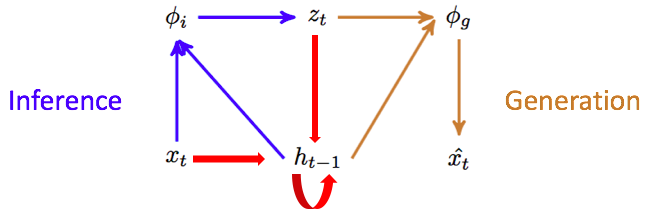 This shows the encoding, decoding, and recurrence of the VRNN at a single time-step.
At each time step \(t\), you sample your latent variable \(z_t^i\) using an encoder that is conditioned off of your data at that time-step \(x_t^i\) and the last hidden state of an RNN
$$ z^i_t = f_{enc}(x^i_t, h_{t-1}) $$You then sample your reconstruction using a decoder that is conditioned off the latent variable and the last hidden state
$$ \hat{x}^i_t = f_{dec}(z^i_t, h_{t-1}) $$The latest hidden state is then conditioned of the data and the latent variable
$$ h_t = f_{RNN}(z^i_t, x_t^i, h_{t-1}) $$Note: For details on the VRNN, see this paper. For more details on the VAE, see its original paper or this phenomenal, more in-depth tutorial.
As \(z_t^i\) values model our data well, we thought this would be a good representation to use for learning a classifier \(G_y\) for our source domain labels \(y_i\). We found that using \(z_T^i\) worked best, where \(T\) corresponds to a data point’s last time-step. In order to make it so this representation could be applied to our target domain, we needed to add a regularizer \(\mathcal{R}(\theta_e)\) to the VRNN (more specifically, the VRNN’s encoder as it generates \(z\)) so that the \(z\) generated would also be applicable to our target domain. We try to minimize:
\[\frac{1}{n} \sum_{i=1}^n \frac{1}{T^i}\mathcal{L}_r(\mathbf{x^i}; \theta_e, \theta_g) + \frac{1}{n} \sum_{i=1}^n \mathcal{L}_y(\mathbf{x^i}; \theta_y,\theta_e) + \lambda \mathcal{R}(\theta_e)\]Here, \(\lambda\) is a tradeoff for regularlizer, \(\theta_e, \theta_g\) are parameters for the VRNN’s encoder and decoder, respectively, and \(\theta_y\) is the parameters for \(G_y\). \(\mathcal{L}_r\) is the vartional lower bound for the VRNN (not discussed here but found in our paper) and \(\mathcal{L}_y\) is a categorical cross-entropy loss function.
Adversarial Training
For our regularizer, we used a domain classification network \(G_d\) that classifies pseudo-labels \(d_i\) for each data point corresponding to which domain they belong to. It has a corresponding categorical cross-entropy loss function \(\mathcal{L}_d\). This is inspired by previous work in domain adaptation that attempts to reduce the domain discrepenacy between the source and target domains. Ben-David has argued (see this paper) that good representations for domain adaptation are those that do not aid in discrimination between domains. In order to make our \(z_T^i\) such that it does not aid in discrimination between domains, we also train a domain classifier using \(z_T^i\). However, instead of trying to minimize the classification error \(\mathcal{L}_d\) we try to maximize it by feeding negative gradients from domain classification to the VRNN’s encoder:
\[\theta_e \leftarrow \theta_e +\eta\lambda\frac{\partial \mathcal{L}_d}{ \partial \theta_d}\]where \(\eta\) is a learning rate for gradient descent. This acts to update its parameters such that they produce a representation that make domain classification more difficult. This network and the encoder then work adversarially: the VRNN producing \(z_T^i\) increasingly more difficult to distinguish domains and the \(G_d\) becoming more competent at classifying \(d_i\). From this process, \(z_T^i\) emerges capturing domain-invariant temporal dependencies.
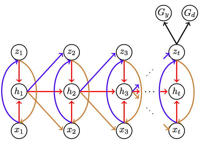 This is a schematic of our model rolled out over time.
Now, we classify all \(z_T^i\) with \(G_d\), and \(z_T^i\) corresponding to \(x_{\mathcal{S}}^i\) strictly with \(G_y\). This leads to the following objectve function which we minimize: \(\underbrace{ \frac{1}{N} \sum_{i=1}^N \frac{1}{T^i}\mathcal{L}_r(\mathbf{x^i}; \theta_e,\theta_g) }_{\text{variational loss}} + \underbrace{ \frac{1}{n} \sum_{i=1}^n \mathcal{L}_y(\mathbf{x^i}; \theta_e,\theta_y) }_{\text{Classification loss}} - \overbrace{ \lambda ( \underbrace{\frac{1}{n} \sum_{i=1}^n \mathcal{L}_d(\mathbf{x^i}; \theta_e,\theta_d) }_{\text{Domain loss for source}} + \underbrace{ \frac{1}{n'} \sum_{i=n+1}^{N} \mathcal{L}_d(\mathbf{x^i}; \theta_e,\theta_d)) }_{\text{Domain loss for target}} }^{\text{Maximizing loss}}\)
where \(\mathcal{L}_d\) is a categorical cross-entropy loss function for domain classifier.
Experiments
As a case study, we performed domain adaptation across age groups. We trained our model to learn to predict mortality from Acute Hypoxemic Respiratory Failure (AHRF) for patients admitted into an ICU using 20 time-series features. We divided patients into 5 age groups
- Group 1: children (0 to 19 yrs, 398 patients)
- Group 2: working-age adult (20 to 45 yrs, 508 patients)
- Group 3: old working-age adult (46 to 65 yrs, 1888 patients)
- Group 4: elderly (66 to 85 yrs, 2394 patients)
- Group 5: old elderly (85 yrs and up, 437 patients)
and performed domain adaptation across different groups (e.g. learning to predict mortality for Group 5 and applying it to Group 1). Below are our results
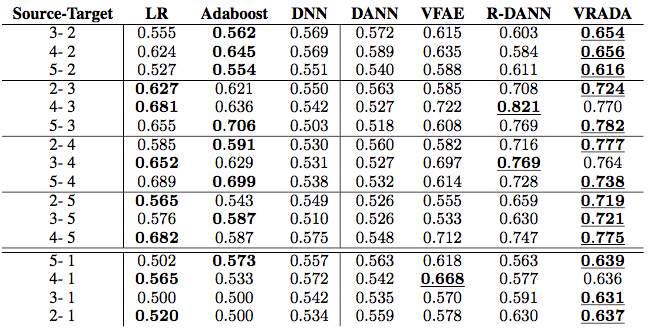
I won’t go into details but just point out a few things. On the left hand side are models that didn’t perform domain adaptation which performed significantly worse. Of models that did, ours performed best by a margin of 4%-6%. You can read more in the paper ;). The analyze the source of our efficacy we studied the latent representations learned by our model and the cell firing patterns of our RNN.
Learned Latent Representations
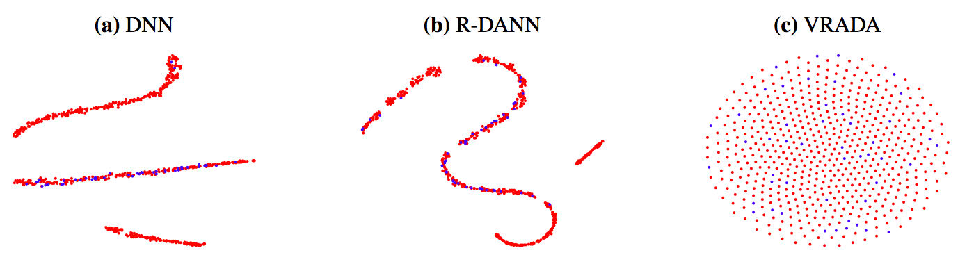 This is a t-sne project of the latent representation of a deep neural network (DNN), a recurrent domain adversarial neural network (R-DANN, a competing domain adaptation model), and VRADA. Red corresponds to source data points and blue to target.
We studied the latent representations learned by our model and competing models to see source and target data were distributed by each model. As stated before, a good representation for domain adaptation is one in which the domain cannot be discerned easily. While blue and red are clustered together for all 3 models, VRADA mixes best. For DNN and R-DANN, there are clusters that are strictly red (source). For VRADA source and target are evenly spread and it is hard to find cluster with strictly one domain. This mixing implies the representations come from the same distribution, i.e. are domain-invariant. We see that better temporal model, e.g. accounting for factors of variation, helps with creating a domain-invariant representation.
Transferring Temporal Dependencies
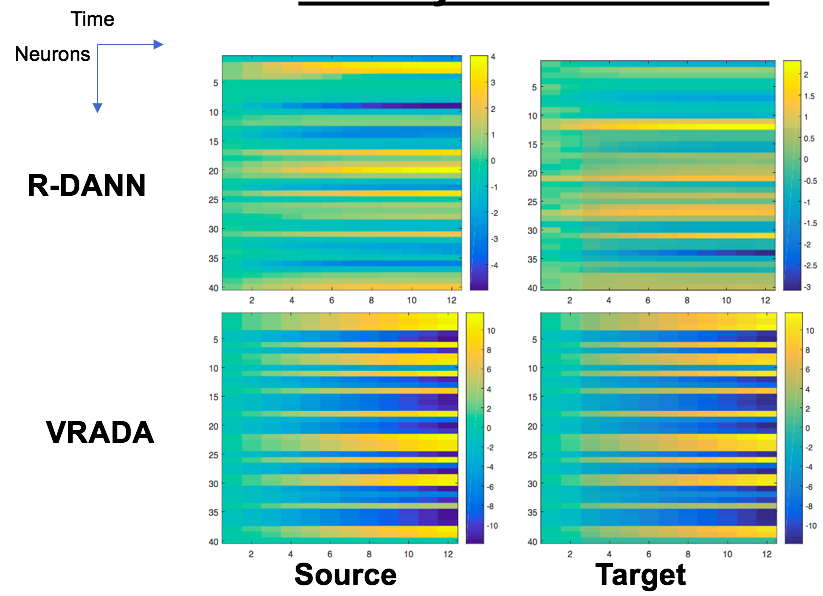 These are the cell firing patterns of the RNN used by our model. The vertical axis corresponds to neurons and the horizontal to a time-step. So the cell corresponding to 4th row and the 3rd column is the firing rate of the 4th neuron at the 3rd time-step.
With both R-DANN and VRADA (both models that create domain-invariant representations), we see high regularity in the firing patterns across domains. However, we can see that accounting for hidden factors of variation when creating domain-invariant representations leads to high consistency in the firing rates across domains. This implies that the temporal dependencies learned for the source domain were transferred to the target domain.
All results showed that creating domain-invariant latent representations and accounting for hidden factors of variation act synergestically. We hope this model serves as a bedrock for future work capturing and transferring temporal tependencies via domain-invariant latent representations.